[Git][debian-gis-team/pysal][master] 7 commits: New upstream version 1.14.4
Bas Couwenberg
gitlab at salsa.debian.org
Thu Jul 19 06:46:57 BST 2018
Bas Couwenberg pushed to branch master at Debian GIS Project / pysal
Commits:
5250889e by Bas Couwenberg at 2018-07-19T06:56:13+02:00
New upstream version 1.14.4
- - - - -
92f753f1 by Bas Couwenberg at 2018-07-19T06:56:31+02:00
Merge tag 'upstream/1.14.4'
Upstream version 1.14.4
- - - - -
9c566ff6 by Bas Couwenberg at 2018-07-19T06:57:03+02:00
New upstream release.
- - - - -
f953a0e6 by Bas Couwenberg at 2018-07-19T06:57:46+02:00
Drop test_examples.patch, applied upstream.
- - - - -
0ea76471 by Bas Couwenberg at 2018-07-19T07:25:48+02:00
Add overrides for package-contains-documentation-outside-usr-share-doc.
- - - - -
e65b9cd5 by Bas Couwenberg at 2018-07-19T07:25:48+02:00
Add lintian override for python-module-in-wrong-location.
- - - - -
f747cb71 by Bas Couwenberg at 2018-07-19T07:25:48+02:00
Set distribution to unstable.
- - - - -
28 changed files:
- LICENSE.txt
- + MIGRATING.md
- debian/changelog
- − debian/patches/series
- − debian/patches/test_examples.patch
- + debian/python-pysal.lintian-overrides
- + debian/python3-pysal.lintian-overrides
- doc/source/conf.py
- doc/source/developers/release.rst
- doc/source/index.rst
- doc/source/references.rst
- doc/source/users/tutorials/econometrics.rst
- pysal/__init__.py
- pysal/cg/kdtree.py
- pysal/contrib/viz/mapping.py
- pysal/contrib/viz/mapping_guide.ipynb
- pysal/contrib/viz/plot.py
- + pysal/contrib/viz/tests/test_plot.py
- pysal/esda/moran.py
- pysal/esda/smoothing.py
- pysal/esda/tests/test_smoothing.py
- pysal/examples/networks/README.md
- pysal/version.py
- pysal/weights/Distance.py
- pysal/weights/_contW_binning.py
- pysal/weights/tests/test_util.py
- pysal/weights/util.py
- setup.py
Changes:
=====================================
LICENSE.txt
=====================================
--- a/LICENSE.txt
+++ b/LICENSE.txt
@@ -11,9 +11,7 @@ modification, are permitted provided that the following conditions are met:
notice, this list of conditions and the following disclaimer in the
documentation and/or other materials provided with the distribution.
-* Neither the name of the GeoDa Center for Geospatial Analysis and Computation
- nor the names of its contributors may be used to endorse or promote products
- derived from this software without specific prior written permission.
+* Neither the name of the PySAL Developers nor the names of its contributors may be used to endorse or promote products derived from this software without specific prior written permission.
THIS SOFTWARE IS PROVIDED BY THE COPYRIGHT HOLDERS AND
CONTRIBUTORS "AS IS" AND ANY EXPRESS OR IMPLIED WARRANTIES,
=====================================
MIGRATING.md
=====================================
--- /dev/null
+++ b/MIGRATING.md
@@ -0,0 +1,278 @@
+# Migrating to PySAL 2.0
+
+<div align='left'>
+
+</div>
+
+PySAL, the Python spatial analysis library, will be changing its package structure.
+
+- We are changing the module structure to better reflect *what you do* with the library rather than the *academic disciplines* the components of the library come from.
+
+- This also makes the library significantly more maintainable for us, since it reduces the bulk of the library and more evenly distributes the load for maintainers.
+
+- As an added benefit, we will release these components, called *submodules*, independently. This lets end users only install components they need, which is helpful for our colleagues in restricted data centers.
+
+- **the main reason** we are doing this, though, is so we can implement new features in an easier fashion, maintain existing features more easily, and solicit new contributions and modules with less friction.
+
+#### The Long & Short of it
+Practially speaking, this means that `pysal` is a single *source redistribution* of many separately-maintained packages, called `submodules`. Each of these submodules are available by themselves on `PyPI`. They are maintained by individuals more closely tied to their code base, and are released on their own schedule. Every six months, the main maintainers of PySAL will collate, test, and re-distribute a stable version of these submodules. The single source release is intended to support our re-packagers, like OSGeoLIVE, Debian, and Conda, as well as most end users. Each *subpackage*, the individual components available on PyPI, are the locus of development, and are pushed forward (or created anew) by their specific maintainers on their respective repositories. For developers interested in minimizing their dependency requirements, it is possible to depend on each `subpackage` alone.
+
+### The Structure of PySAL 2.0
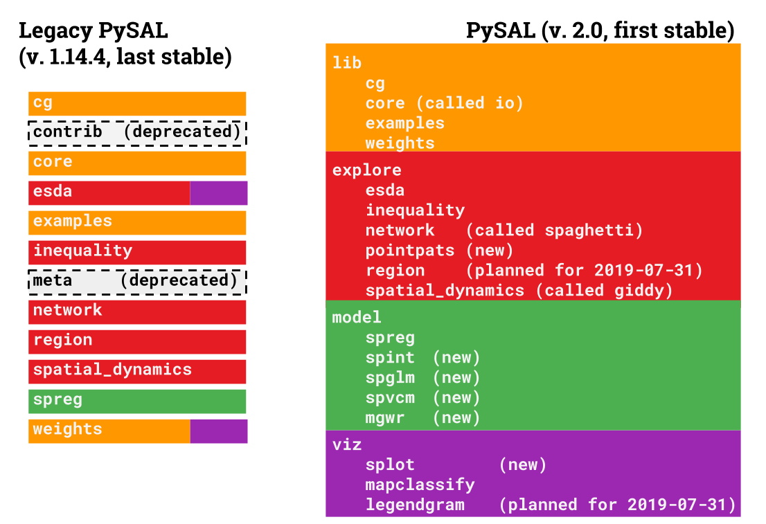
+To make this happen, we must re-arrange some existing functionality in the library so that it can be packaged separately. In total, `pysal` 2.0 will be organized with five main thematic modules with the following functionality:
+
+* `lib`: core functionality used by other modules to work with spatial data in Python, including:
+ - the construction of graphs (also known as spatial weights) from spatial data
+ - computational geometry algorithms:
+ + alpha shapes
+ + quadtrees, rTrees, & spherical KDTrees
+ + methods to construct graphs from `scipy` Delaunay triangulation objects
+ + Pure Python data structures to represent planar geometric objects
+ - pure Python readers/writers for graph/spatial weights files and some spatial data types
+* `explore`: exploratory spatial data analysis of clusters, hotspots, and spatial outliers, plus spatial statistics on graphs and point patterns. These include
+ * Point pattern analysis of centrography and colocation ($F$,$G$,$J$,$K$ statistics in space)
+ * Pattern analysis of point patterns snapped to a network ($F$,$G$,$K$ statistics on networks)
+ * Analysis of spatial patterning on lattices, including
+ * univariate Join count statistics
+ * Moran's $I$ statistics, including local & bivariate methods
+ * Geary's $C$
+ * Getis-Ord $G$, $G^*$, and local $G$ statistics
+ * General $\Gamma$ statistics for spatial clustering
+ * methods to construct & analyze the space-time dynamics and distributions of data, including Markov models and distributional dynamics statistics
+* `model`: explicitly spatial modeling tools including:
+ - geographically-weighted regression, a generalized additive spatial model specification for local coefficients
+ - spatially-correlated variance-components models, a type of Bayesian hierarchical model providing for group-level spatial mixed effects, as well as diagnostics for Bayesian modeling (Geweke, Markov Chain Monte Carlo Standard Error, Potential Scale Reduction Factors)
+ - Bayesian spatially-varying coefficient process models (e.g. local random effects models)
+ - Maximum Likelihood spatial econometric models, including:
+ + mixed regressive-autoregressive (spatial lag) model
+ + spatially-correlated error models
+ + spatial regimes/spatial mixture models
+ + seemingly-unrelated regression models
+ + combinations of these various effects
+ - econometric specification testing methods, including spatial Lagrange Multiplier, Anselin-Kelejian, Chow, and Jarque-Bera tests.
+- `viz`: methods to visualize and analyze spatial datasets, specifically the output of exploratory spatial statistics.
+
+This document provides a brief overview of what each of the new modules are, how they relate to the last **legacy** version of `pysal`, version `1.14.4`, and what you need to do in order to keep your code running the way you expect.
+
+# Porting your code
+
+The changes in `pysal` collect together modules that are used for a similar purpose:
+
+
+
+Many things are new in `pysal` 2.0. In order to ensure we can keep making new things easily and maintain what we have, we've released each of the *submodules* (those underneath `model`,`viz`, and `explore`) as their own python packages on PyPI. We will also release the `lib` module as its own package, `libpysal`, on PyPI.
+
+This means that new users can make new submodules by following our [submodule contract](https://github.com/pysal/pysal/wiki/Submodule-Contract). Further, contributors should make pull requests to the submodules directly, not to [`pysal/pysal`](https://github.com/pysal/pysal).
+
+## using the standard `pysal` for a stable six-month release cycle
+
+If you want to keep your usual stable `pysal` dependency, it is sufficient to update your imports according to the mappings we provide in the [**Module Lookup**](#module-lookup) section. `pysal` will continue to stick to regular 6-month releases put out by multiple maintainers, with bug-fix releases as needed throughout the year.
+
+This version will still have nightly regression testing run and will be ensured to work with the latest releases of `numpy` and `scipy`. If you don't have an urgent need to reduce your dependency size or the availability of PySAL, continuing to depend on `pysal` directly is the right choice.
+
+## using the appropriate sub-module for fresher releases & more stable dependencies
+
+If you only use one contained part of `pysal`, are interested in developing another statistical analysis package that only depends on `libpysal`, or simply want to keep your build as lean as possible, you can also install only the sub-modules you require, independently of `pysal`. This is the best option for those of you in restricted analysis environments where every line of code must be vetted by an expert, such as users in restricted data centers conducting academic work.
+
+**To preview these changes, install the `pysalnext` package using `pip`. If your package works with `pysalnext`, it should work on `pysal` 2.0.**
+
+All of the sub-packages included in `pysalnext` contain a significant amount of new functionality, as well as interoperability tools for other packages, such as `networkx` and `geopandas`. In addition, most of the old tools from `pysal` are reorganized. In total, there are `12` distinct packages in `pysalnext`, with more being added often. These packages are:
+- `libpysal`: the core of the library, containing computational geometry, graph construction, and read/write tools.
+- `esda`: the exploratory spatial data analysis toolkit, containing many statistical functions for characterizing spatial patterns.
+- `pointpats`: methods and statistical functions to statistically analyze spatial clustering in point patterns
+- `spaghetti`: methods and statistical functions to analyze geographic networks, including the statistical distribution of points on network topologies.
+- `giddy`: the geospatial distribution dynamics package, designed to study and characterize how distributions change and relate over space and time.
+- `mapclassify`: a package with map classification algorithms for cartography
+- `splot`: a collection of statistical visualizations for the analysis methods included across `pysalnext`
+- `gwr`: geographically-weighted regression (both single- and multi-scale)
+- `spglm`: methods & functions to fit sparse GLMs
+- `spint`: spatial interaction models
+- `spreg`: spatial econometric regression
+- `spvcm`: spatially-correlated variance components models, plus diagnostics and plotting for Bayesian models fit in `pysalnext`.
+
+There are four main changes that have occurred in `pysalnext`. From legacy `pysal`, these are:
+
+1. `pysal.contrib`: removed due to lack of unittesting and heterogeneous code quality; moved to independent modules where possible.
+
+2. `pysal.esda.smoothing`: removed due to intractable and subtle numerical bugs in the code caused by porting to Python 3. There is an effort to re-implement this in Python, and will be added when/if this effort finishes.
+
+3. `pysal.region`: removed because the new version has significantly more dependencies, including `pulp` and `scikit-learn`. Grab this as a standalone package using `pip install region`.
+
+4. `pysal.meta`: removed.
+
+If you'd like to get code from submodules, they usually have a one-to-one replacement. This will be discussed later in the [**Module Lookup**](#Module-Lookup) section.
+
+# Module Lookup
+
+Here is a list of the locations of all of the commonly-used modules in legacy `pysal`, and where they will move in the next release of `pysal`.
+
+**To preview these changes, install the `pysalnext` package using `pip`. If your package works with `pysalnext`, it should work on `pysal` 2.0. **
+
+### Modules in `libpysal`:
+- `pysal.cg` will change to `pysal.lib.cg`
+- `pysal.weights` will change to `pysal.lib.weights`, and many weights construction classes now have `from_geodataframe` methods that can graphs directly from `geopandas` `GeoDataFrames`.
+- `pysal.open` will change to `pysal.lib.io.open`, and most of `pysal.core` will move to `pysal.lib.io`. *Note: using* `pysal.lib.io.open`*for **anything** but reading/writing spatial weights matrices/graphs is not advised. Please migrate to* `geopandas`* for all spatial data read/write. Further, note that* `WeightsConverter` *has also been deprecated; if you need to convert weights, do so manually using sequential* `open`* and *`write`* statements.*
+- `pysal.examples` will change to `pysal.lib.examples`
+### Modules from `spatial_dynamics`
+`pysal.spatial_dynamics` will change to `pysal.explore.giddy`
+
+### Modules from `inequality`
+
+`pysal.inequality` will change to `pysal.explore.inequality`
+
+### Modules from `esda`:
+These will mainly move into `pysal.explore.esda`, except for `smoothing` and `mixture_smoothing` (which will be deprecated) and `mapclassify`, which will move to `pysal.viz.mapclassify`.
+### Modules from `network`:
+These will move directly into `pysal.explore.spaghetti`
+### Modules from `inequality`:
+`pysal.inequality` has been published as its own package, `inequality`, and moved to `pysal.explore.inequality`.
+### Modules from `spreg`:
+`pysal.spreg` has been moved wholesale into `pysal.model.spreg`, which now contains many additional kinds of spatial regression models, including spatial interaction, Bayesian multilevel, and geographically-weighted regression methods.
+
+## Examples
+
+#### Reading/Writing Data:
+
+```python
+import pysal
+file_handler = pysal.open(pysal.examples.get_path('columbus.dbf'))
+data = np.asarray(file_handler.by_col('HOVAL'))
+```
+
+becomes:
+
+```python
+import geopandas
+from pysal.lib import examples
+dataframe = geopandas.read_file(examples.get_path('columbus.dbf'))
+data = data['HOVAL'].values
+```
+
+#### Reading/Writing Graphs or Spatial Weights:
+
+```python
+import pysal
+graph = pysal.open(pysal.examples.get_path('columbus.gal')).read()
+```
+
+becomes
+
+```python
+from pysal.lib import weights, examples
+graph = weights.W.from_file(examples.get_path('columbus.gal'))
+```
+
+or, building directly on top of the developer-focused `libpysal` package:
+
+```python
+from libpysal import weights, examples
+graph = weights.W.from_file(examples.get_path('columbus.gal'))
+```
+
+#### Making map classifications
+
+```python
+from pysal.esda.mapclassify import Jenks_Caspall
+Jenks_Caspall(your_data).yb
+```
+
+becomes
+
+```python
+from pysal.viz import mapclassify
+labels = mapclassify.Jenks_Caspall(features).yb
+```
+
+Or, built directly on top of the developer-focused package `mapclassify`, which may have newer features in the future:
+
+```python
+import mapclassify
+labels = mapclassify.Jenks_Caspall(features).yb
+```
+
+
+
+#### Fitting a spatial regression:
+
+```python
+import pysal
+file_handler = pysal.open(pysal.examples.get_path('columbus.dbf'))
+y = np.asarray(file_handler.by_col('HOVAL'))
+X = file_handler.by_col_array(['CRIME', 'INC'])
+graph = pysal.queen_from_shapefile(pysal.examples.get_path('columbus.shp'))
+model = pysal.spreg.ML_Lag(y,X, w=graph,
+ name_x = ['CRIME', 'INC'],
+ name_y = 'HOVAL')
+```
+
+becomes
+
+```python
+from pysal.model import spreg
+from pysal.lib import weights, examples
+import geopandas
+dataframe = geopandas.read_file(examples.get_path("columbus.dbf"))
+graph = weights.Queen.from_dataframe(dataframe) # Queen.from_shapefile also supported
+model = spreg.ML_Lag(dataframe[['HOVAL']].values,
+ dataframe[['CRIME', 'INC']].values,
+ name_x = ['CRIME', 'INC'], name_y = 'HOVAL')
+```
+
+Or, building on top of the standalone `spreg` package, which may have new bugfixes or compatibility options in the future:
+
+```python
+from pysal.model import spreg
+from pysal.lib import weights, examples
+import geopandas
+dataframe = geopandas.read_file(examples.get_path("columbus.dbf"))
+graph = weights.Queen.from_dataframe(dataframe)
+model = spreg.ML_Lag(dataframe[['HOVAL']].values,
+ dataframe[['CRIME', 'INC']].values,
+ name_x = ['CRIME', 'INC'], name_y = 'HOVAL')
+model2 = spreg.ML_Lag.from_formula('HOVAL ~ CRIME + INC',
+ data=dataframe)
+```
+
+#### Computing a Moran statistic:
+
+```python
+import pysal
+file_handler = pysal.open(pysal.examples.get_path('columbus.dbf'))
+y = np.asarray(file_handler.by_col('HOVAL'))
+graph = pysal.open(pysal.examples.get_path('columbus.gal')).read()
+moran_stat = pysal.Moran(y,graph)
+print(moran_stat.I, moran_stat.p_z_sim)
+```
+
+becomes
+
+```python
+from pysal.explore import esda
+from pysal.lib import weights, examples
+import geopandas
+dataframe = geopandas.read_file(examples.get_path("columbus.dbf"))
+graph = weights.Queen.from_dataframe(dataframe)
+moran_stat = esda.Moran(dataframe['HOVAL'], graph)
+print(moran_stat.I, moran_stat.p_z_sim)
+```
+
+or, building directly off of the developer-focused package `esda` , which may have features not yet available in `pysal` itself:
+
+```python
+import esda
+from pysal.lib import weights, examples
+import geopandas
+dataframe = geopandas.read_file(examples.get_path("columbus.dbf"))
+graph = weights.Queen.from_dataframe(dataframe)
+moran_stat = esda.Moran(dataframe['HOVAL'], graph, fancy_new_option=True)
+print(moran_stat.I, moran_stat.p_z_sim)
+```
+
+
+
+# I really don't want to change anything; what can I do?
+
+<font color='red'><bf>This is not recommended.</bf></font>
+
+For a longer change window, feel free to `import pysal._legacy as pysal`. We urge you to not do this, since we plan on deprecating this as well. If you can make the changes described above, you will have a much more stable and future-proof API. We feel these changes are reasonable and will greatly enhance how easy it is for us to maintain `pysal` and move new functionality forward.
+
+### Please contact us on [gitter](https://gitter.com/pysal/pysal) if there are any remaining concerns or questions, and for help or advice.
\ No newline at end of file
=====================================
debian/changelog
=====================================
--- a/debian/changelog
+++ b/debian/changelog
@@ -1,13 +1,18 @@
-pysal (1.14.3-2) UNRELEASED; urgency=medium
+pysal (1.14.4-1) unstable; urgency=medium
+ * Team upload.
+ * New upstream release.
* Update copyright-format URL to use HTTPS.
* Update Vcs-* URLs for Salsa.
* Bump Standards-Version to 4.1.5, no changes.
* Drop ancient X-Python-Version field.
* Strip trailing whitespace from control & rules files.
* Use filter instead of findstring to prevent partial matches.
+ * Drop test_examples.patch, applied upstream.
+ * Add overrides for package-contains-documentation-outside-usr-share-doc.
+ * Add lintian override for python-module-in-wrong-location.
- -- Bas Couwenberg <sebastic at debian.org> Sun, 21 Jan 2018 10:32:03 +0100
+ -- Bas Couwenberg <sebastic at debian.org> Thu, 19 Jul 2018 06:58:36 +0200
pysal (1.14.3-1) unstable; urgency=medium
=====================================
debian/patches/series deleted
=====================================
--- a/debian/patches/series
+++ /dev/null
@@ -1 +0,0 @@
-test_examples.patch
=====================================
debian/patches/test_examples.patch deleted
=====================================
--- a/debian/patches/test_examples.patch
+++ /dev/null
@@ -1,30 +0,0 @@
-Description: Fix UnicodeDecodeError by changing UTF-8 character to ASCII.
- ======================================================================
- ERROR: test_parser (pysal.examples.test_examples.Example_Tester)
- ----------------------------------------------------------------------
- Traceback (most recent call last):
- File "/build/pysal-1.14.3/.pybuild/pythonX.Y_3.6/build/pysal/examples/test_examples.py", line 15, in test_parser
- self.extext = ex.explain(example)
- File "/build/pysal-1.14.3/.pybuild/pythonX.Y_3.6/build/pysal/examples/__init__.py", line 77, in explain
- return _read_example(fpath)
- File "/build/pysal-1.14.3/.pybuild/pythonX.Y_3.6/build/pysal/examples/__init__.py", line 55, in _read_example
- title = io.readline().strip('\n')
- File "/usr/lib/python3.6/encodings/ascii.py", line 26, in decode
- return codecs.ascii_decode(input, self.errors)[0]
- UnicodeDecodeError: 'ascii' codec can't decode byte 0xe3 in position 384: ordinal not in range(128)
- -------------------- >> begin captured stdout << ---------------------
-Author: Bas Couwenberg <sebastic at debian.org>
-Forwarded: https://github.com/pysal/pysal/pull/1002
-Applied-Upstream: https://github.com/pysal/pysal/commit/8d1e59649d2ee14f5499ed5ba68d99e32fea89f8
-
---- a/pysal/examples/networks/README.md
-+++ b/pysal/examples/networks/README.md
-@@ -9,7 +9,7 @@ Datasets used for network testing
- * eberly_net.shx: spatial index.
- * eberly_net_pts_offnetwork.dbf: attribute data for points off network. (k=2)
- * eberly_net_pts_offnetwork.shp: Point shapefile. (n=100)
--* eberly_net_pts_offnetwork.shx: spatial index。
-+* eberly_net_pts_offnetwork.shx: spatial index.
- * eberly_net_pts_onnetwork.dbf: attribute data for points on network. (k=1)
- * eberly_net_pts_onnetwork.shp: Point shapefile. (n=110)
- * eberly_net_pts_onnetwork.shx: spatial index.
=====================================
debian/python-pysal.lintian-overrides
=====================================
--- /dev/null
+++ b/debian/python-pysal.lintian-overrides
@@ -0,0 +1,3 @@
+# README files are parsed by the code.
+package-contains-documentation-outside-usr-share-doc usr/lib/python*/dist-packages/pysal/examples/*
+
=====================================
debian/python3-pysal.lintian-overrides
=====================================
--- /dev/null
+++ b/debian/python3-pysal.lintian-overrides
@@ -0,0 +1,6 @@
+# README files are parsed by the code.
+package-contains-documentation-outside-usr-share-doc usr/lib/python*/dist-packages/pysal/examples/*
+
+# False positive? dh_python3 should do the right thing.
+python-module-in-wrong-location usr/lib/python3.*/dist-packages/pysal/* usr/lib/python3/dist-packages/pysal/*
+
=====================================
doc/source/conf.py
=====================================
--- a/doc/source/conf.py
+++ b/doc/source/conf.py
@@ -47,9 +47,9 @@ copyright = u'2014-, PySAL Developers; 2009-13 Sergio Rey'
# built documents.
#
# The short X.Y version.
-version = '1.14.3'
+version = '1.14.4'
# The full version, including alpha/beta/rc tags.
-release = '1.14.3'
+release = '1.14.4'
# The language for content autogenerated by Sphinx. Refer to documentation
# for a list of supported languages.
=====================================
doc/source/developers/release.rst
=====================================
--- a/doc/source/developers/release.rst
+++ b/doc/source/developers/release.rst
@@ -14,21 +14,19 @@ Prepare the release
$ python tools/github_stats.py days >> chglog
-- where `days` is the number of days to start the logs at
-- Prepend `chglog` to `CHANGELOG` and edit
+- where `days` is the number of days to start the logs at.
+- Prepend `chglog` to `CHANGELOG` and edit.
- Edit THANKS and README and README.md if needed.
-- Edit the file `version.py` to update MAJOR, MINOR, MICRO
+- Edit the file `version.py` to update MAJOR, MINOR, MICRO.
- Bump::
$ cd tools; python bump.py
- Commit all changes.
-- Push_ your branch up to your GitHub repos
+- Push_ your branch up to your GitHub repos.
- On github issue a pull request, with a target of **upstream master**.
Add a comment that this is for release.
-
-
Make docs
---------
@@ -37,18 +35,18 @@ As of version 1.6, docs are automatically compiled and hosted_.
Make a source dist and test locally (Python 3)
----------------------------------------------
-On each build machine
+On each build machine::
- $ git clone http://github.com/pysal/pysal.git
- $ cd pysal
- $ python setup.py sdist
- $ cp dist/PySAL-1.14.2.tar.gz ../junk/.
- $ cd ../junk
- $ conda create -n pysaltest3 python=3 pip
- $ source activate pysaltest3
- $ pip install PySAL-1.14.2.tar.gz
- $ rm -r /home/serge/anaconda3/envs/pysaltest3/lib/python3.6/site-packages/pysal/contrib
- $ nosetests /home/serge/anaconda3/envs/pysaltest3/lib/python3.6/site-packages/pysal/
+ $ git clone http://github.com/pysal/pysal.git
+ $ cd pysal
+ $ python setup.py sdist
+ $ cp dist/PySAL-1.14.2.tar.gz ../junk/.
+ $ cd ../junk
+ $ conda create -n pysaltest3 python=3 pip nose nose-progressive nose-exclude
+ $ source activate pysaltest3
+ $ pip install PySAL-1.14.2.tar.gz
+ $ rm -r /home/serge/anaconda3/envs/pysaltest3/lib/python3.6/site-packages/pysal/contrib
+ $ nosetests /home/serge/anaconda3/envs/pysaltest3/lib/python3.6/site-packages/pysal/
You can modify the above to test for Python 2 environments.
@@ -56,17 +54,19 @@ You can modify the above to test for Python 2 environments.
Upload release to pypi
----------------------
-- Make and upload_ to the Python Package Index in one shot!::
+- Make and upload_ to the `Python Package Index`_ in one shot!::
+
+ $ python setup.py sdist upload
+
+ - if not registered_, do so by following the prompts::
- $ python setup.py sdist upload
+ $ python setup.py register
- - if not registered_, do so. Follow the prompts. You can save the
- login credentials in a dot-file, .pypirc
+ - You can save the login credentials in a dot-file, `.pypirc`.
-- Make and upload the Windows installer to SourceForge.
- - On a Windows box, build the installer as so::
+- Make and upload the Windows installer to SourceForge_. On a Windows box, build the installer as so::
- $ python setup.py bdist_wininst
+ $ python setup.py bdist_wininst
Create a release on github
--------------------------
@@ -77,26 +77,29 @@ https://help.github.com/articles/creating-releases/
Announce
--------
-- Draft and distribute press release on openspace-list, pysal.org, spatial.ucr.edu
+- Draft and distribute press release on openspace-list, pysal.org, `spatial.ucr.edu`_ .
Bump master version
-------------------
-- Change MAJOR, MINOR version in setup script.
-- Change pysal/version.py to dev number
-- Change the docs version from X.x to X.xdev by editing doc/source/conf.py in two places.
-- Update the release schedule in doc/source/developers/guidelines.rst
+- Change MAJOR, MINOR version in `setup.py`.
+- Change `pysal/version.py`.
+- Change the docs version by editing `doc/source/conf.py` in two places (version and release).
+- Update the release schedule in `doc/source/developers/guidelines.rst`.
Update the `github.io news page <https://github.com/pysal/pysal.github.io/blob/master/_includes/news.md>`_
-to announce the release.
+to announce the release.
-.. _upload: http://docs.python.org/2.7/distutils/uploading.html
-.. _registered: http://docs.python.org/2.7/distutils/packageindex.html
+.. _upload: https://docs.python.org/2.7/distutils/packageindex.html#the-upload-command
+.. _registered: https://docs.python.org/2.7/distutils/packageindex.html#the-register-command
.. _source: http://docs.python.org/distutils/sourcedist.html
-.. _hosted: http://pysal.readthedocs.org
+.. _hosted: http://pysal.readthedocs.io/en/latest/users/index.html
.. _branch: https://github.com/pysal/pysal/wiki/GitHub-Standard-Operating-Procedures
.. _policy: https://github.com/pysal/pysal/wiki/Example-git-config
.. _create the release: https://help.github.com/articles/creating-releases/
.. _Push: https://github.com/pysal/pysal/wiki/GitHub-Standard-Operating-Procedures
+.. _Python Package Index: https://pypi.python.org/pypi/PySAL
+.. _SourceForge: https://sourceforge.net
+.. _spatial.ucr.edu: http://spatial.ucr.edu/news.html
=====================================
doc/source/index.rst
=====================================
--- a/doc/source/index.rst
+++ b/doc/source/index.rst
@@ -20,8 +20,8 @@ PySAL
.. sidebar:: Releases
- - `Stable 1.14.3 (Released 2017-11-2) <users/installation.html>`_
- - `Development <http://github.com/pysal/pysal/tree/dev>`_
+ - `Stable 1.14.4 (Released 2018-07-17) <users/installation.html>`_
+ - `Development <http://github.com/pysal/pysal/tree/master>`_
PySAL is an open source library of spatial analysis functions written in
Python intended to support the development of high level applications.
=====================================
doc/source/references.rst
=====================================
--- a/doc/source/references.rst
+++ b/doc/source/references.rst
@@ -10,7 +10,7 @@ References
.. [Anselin1997] Anselin, L. and Kelejian, H. H. (1997). Testing for spatial error autocorrelation in the presence of endogenous regressors. International Regional Science Review, 20(1-2):153–182.
.. [Anselin2011] Anselin, L. (2011). GMM Estimation of Spatial Error Autocorrelation with and without Heteroskedasticity.
.. [Arraiz2010] Arraiz, I., Drukker, D. M., Kelejian, H. H., and Prucha, I. R. (2010). A spatial Cliff-Ord-type model with heteroskedastic innovations: Small and large sample results. Journal of Regional Science, 50(2):592–614.
-.. [Assuncao1999] Assuncao, R. M. and Reis, E. A. (1999). A new proposal to adjust moran’s i for population density. Statistics in medicine, 18(16):2147–2162.
+.. [Assuncao1999] Assuncao, R. M. and Reis, E. A. (1999). A new proposal to adjust Moran’s I for population density. Statistics in medicine, 18(16):2147–2162.
.. [Baker2004] Baker, R. D. (2004). Identifying space–time disease clusters. Acta tropica, 91(3):291–299.
.. [Belsley1980] Belsley, D. A., Kuh, E., and Welsch, R. E. (1980). Regression diagnostics: Identifying influential data and sources of collinearity, volume 1.
.. [Bickenbach2003] Bickenbach, F. and Bode, E. (2003). Evaluating the Markov property in studies of economic convergence. International Regional Science Review, 26(3):363–392.
=====================================
doc/source/users/tutorials/econometrics.rst
=====================================
--- a/doc/source/users/tutorials/econometrics.rst
+++ b/doc/source/users/tutorials/econometrics.rst
@@ -7,7 +7,7 @@ Spatial Econometrics
Comprehensive user documentation on spreg can be found in
Anselin, L. and S.J. Rey (2014) `Modern Spatial Econometrics in Practice:
A Guide to GeoDa, GeoDaSpace and PySAL.
-<http://www.amazon.com/Modern-Spatial-Econometrics-Practice-GeoDaSpace-ebook/dp/B00RI9I44K>`_
+<http://a.co/aHZnDLW>`_
GeoDa Press, Chicago.
=====================================
pysal/__init__.py
=====================================
--- a/pysal/__init__.py
+++ b/pysal/__init__.py
@@ -46,13 +46,25 @@ try:
pysal.common.pandas = pandas
except ImportError:
pysal.common.pandas = None
-
+
# Load the IOHandlers
from pysal.core import IOHandlers
# Assign pysal.open to dispatcher
open = pysal.core.FileIO.FileIO
-from pysal.version import version
+from pysal.version import version as __version__, new_api_date
+from warnings import warn
+from numpy import VisibleDeprecationWarning
+warn("PySAL's API will be changed on {}. The last "
+ "release made with this API is version {}. "
+ "A preview of the next API version is provided in "
+ "the `pysalnext` package. The API changes and a "
+ "guide on how to change imports is provided "
+ "at https://migrating.pysal.org".format(new_api_date,
+ __version__
+ ), VisibleDeprecationWarning)
+
+# Load the IOHandlers
#from pysal.version import stable_release_date
#import urllib2, json
#import config
=====================================
pysal/cg/kdtree.py
=====================================
--- a/pysal/cg/kdtree.py
+++ b/pysal/cg/kdtree.py
@@ -158,7 +158,11 @@ class Arc_KDTree(temp_KDTree):
distance_upper_bound, self.radius)
d, i = temp_KDTree.query(self, self._toXYZ(x), k,
eps=eps, distance_upper_bound=distance_upper_bound)
- dims = len(d.shape)
+ if isinstance(d, float):
+ dims = 0
+ else:
+ dims = len(d.shape)
+
r = self.radius
if dims == 0:
return sphere.linear2arcdist(d, r), i
=====================================
pysal/contrib/viz/mapping.py
=====================================
--- a/pysal/contrib/viz/mapping.py
+++ b/pysal/contrib/viz/mapping.py
@@ -7,14 +7,11 @@ ToDo:
"""
-__author__ = "Sergio Rey <sjsrey at gmail.com>", "Dani Arribas-Bel <daniel.arribas.bel at gmail.com"
-
-
from warnings import warn
import pandas as pd
import pysal as ps
import numpy as np
-import matplotlib.pyplot as plt
+import matplotlib.pyplot as plt
from matplotlib import colors as clrs
import matplotlib as mpl
from matplotlib.pyplot import fill, text
@@ -22,7 +19,9 @@ from matplotlib import cm
from matplotlib.patches import Polygon
import collections
from matplotlib.path import Path
-from matplotlib.collections import LineCollection, PathCollection, PolyCollection, PathCollection, PatchCollection, CircleCollection
+from matplotlib.collections import (
+ LineCollection, PathCollection, PolyCollection, PathCollection,
+ PatchCollection, CircleCollection)
from color import get_color_map
@@ -30,33 +29,41 @@ try:
import bokeh.plotting as bk
from bokeh.models import HoverTool
except:
- warn('Bokeh not installed. Functionality ' \
- 'related to it will not work')
+ warn('Bokeh not installed. Functionality '
+ 'related to it will not work')
+
+
+__author__ = ("Sergio Rey <sjsrey at gmail.com>",
+ "Dani Arribas-Bel <daniel.arribas.bel at gmail.com")
+
+
# Classifier helper
classifiers = ps.esda.mapclassify.CLASSIFIERS
-classifier = {c.lower():getattr(ps.esda.mapclassify,c) for c in classifiers}
+classifier = {c.lower(): getattr(ps.esda.mapclassify, c) for c in classifiers}
+
def value_classifier(y, scheme='Quantiles', **kwargs):
"""
Return classification for an indexed Series of values
...
- Arguments
- ---------
- y : Series
- Indexed series containing values to be classified
- scheme : str
- [Optional. Default='Quantiles'] Name of the PySAL classifier
- to be used
- **kwargs : dict
- Additional arguments specific to the classifier of choice
- (see the classifier's documentation for details)
+ Parameters
+ ----------
+ y : Series
+ Indexed series containing values to be classified
+ scheme : str
+ [Optional. Default='Quantiles'] Name of the PySAL classifier
+ to be used
+ **kwargs : dict
+ Additional arguments specific to the classifier of choice
+ (see the classifier's documentation for details)
Returns
-------
- labels : Series
- Indexed series containing classes for each observation
- classification : Map_Classifier instance
+ labels : Series
+ Indexed series containing classes for each observation
+ classification : Map_Classifier instance
+
"""
c = classifier[scheme.lower()](y, **kwargs)
return (pd.Series(c.yb, index=y.index), c)
@@ -69,27 +76,25 @@ def map_point_shp(shp, which='all', bbox=None):
Create a map object from a point shape
...
- Arguments
- ---------
-
- shp : iterable
- PySAL point iterable (e.g.
- shape object from `ps.open` a point shapefile) If it does
- not contain the attribute `bbox`, it must be passed
- separately in `bbox`.
- which : str/list
- List of booleans for which polygons of the shapefile to
- be included (True) or excluded (False)
- bbox : None/list
- [Optional. Default=None] List with bounding box as in a
- PySAL object. If nothing is passed, it tries to obtain
- it as an attribute from `shp`.
+ Parameters
+ ----------
+ shp : iterable
+ PySAL point iterable (e.g.
+ shape object from `ps.open` a point shapefile) If it does
+ not contain the attribute `bbox`, it must be passed
+ separately in `bbox`.
+ which : str/list
+ List of booleans for which polygons of the shapefile to
+ be included (True) or excluded (False)
+ bbox : None/list
+ [Optional. Default=None] List with bounding box as in a
+ PySAL object. If nothing is passed, it tries to obtain
+ it as an attribute from `shp`.
Returns
-------
-
- map : PatchCollection
- Map object with the points from the shape
+ map : PatchCollection
+ Map object with the points from the shape
'''
if not bbox:
@@ -104,40 +109,39 @@ def map_point_shp(shp, which='all', bbox=None):
pts.append(pt)
pts = np.array(pts)
sc = plt.scatter(pts[:, 0], pts[:, 1])
- #print(sc.get_axes().get_xlim())
- #_ = _add_axes2col(sc, bbox)
- #print(sc.get_axes().get_xlim())
+ # print(sc.get_axes().get_xlim())
+ # _ = _add_axes2col(sc, bbox)
+ # print(sc.get_axes().get_xlim())
return sc
+
def map_line_shp(shp, which='all', bbox=None):
'''
Create a map object from a line shape
...
- Arguments
- ---------
-
- shp : iterable
- PySAL line iterable (e.g.
- shape object from `ps.open` a line shapefile) If it does
- not contain the attribute `bbox`, it must be passed
- separately in `bbox`.
- which : str/list
- List of booleans for which polygons of the shapefile to
- be included (True) or excluded (False)
- bbox : None/list
- [Optional. Default=None] List with bounding box as in a
- PySAL object. If nothing is passed, it tries to obtain
- it as an attribute from `shp`.
+ Parameters
+ ----------
+ shp : iterable
+ PySAL line iterable (e.g.
+ shape object from `ps.open` a line shapefile) If it does
+ not contain the attribute `bbox`, it must be passed
+ separately in `bbox`.
+ which : str/list
+ List of booleans for which polygons of the shapefile to
+ be included (True) or excluded (False)
+ bbox : None/list
+ [Optional. Default=None] List with bounding box as in a
+ PySAL object. If nothing is passed, it tries to obtain
+ it as an attribute from `shp`.
Returns
-------
-
- map : PatchCollection
- Map object with the lines from the shape
- This includes the attribute `shp2dbf_row` with the
- cardinality of every line to its row in the dbf
- (zero-offset)
+ map : PatchCollection
+ Map object with the lines from the shape
+ This includes the attribute `shp2dbf_row` with the
+ cardinality of every line to its row in the dbf
+ (zero-offset)
'''
if not bbox:
@@ -159,39 +163,38 @@ def map_line_shp(shp, which='all', bbox=None):
rows.append(i)
i += 1
lc = LineCollection(patches)
- #_ = _add_axes2col(lc, bbox)
+ # _ = _add_axes2col(lc, bbox)
lc.shp2dbf_row = rows
return lc
+
def map_poly_shp(shp, which='all', bbox=None):
'''
Create a map object from a polygon shape
...
- Arguments
- ---------
-
- shp : iterable
- PySAL polygon iterable (e.g.
- shape object from `ps.open` a poly shapefile) If it does
- not contain the attribute `bbox`, it must be passed
- separately in `bbox`.
- which : str/list
- List of booleans for which polygons of the shapefile to
- be included (True) or excluded (False)
- bbox : None/list
- [Optional. Default=None] List with bounding box as in a
- PySAL object. If nothing is passed, it tries to obtain
- it as an attribute from `shp`.
+ Parameters
+ ----------
+ shp : iterable
+ PySAL polygon iterable (e.g.
+ shape object from `ps.open` a poly shapefile) If it does
+ not contain the attribute `bbox`, it must be passed
+ separately in `bbox`.
+ which : str/list
+ List of booleans for which polygons of the shapefile to
+ be included (True) or excluded (False)
+ bbox : None/list
+ [Optional. Default=None] List with bounding box as in a
+ PySAL object. If nothing is passed, it tries to obtain
+ it as an attribute from `shp`.
Returns
-------
-
- map : PatchCollection
- Map object with the polygons from the shape
- This includes the attribute `shp2dbf_row` with the
- cardinality of every polygon to its row in the dbf
- (zero-offset)
+ map : PatchCollection
+ Map object with the polygons from the shape
+ This includes the attribute `shp2dbf_row` with the
+ cardinality of every polygon to its row in the dbf
+ (zero-offset)
'''
if not bbox:
@@ -215,34 +218,37 @@ def map_poly_shp(shp, which='all', bbox=None):
rows.append(i)
i += 1
pc = PolyCollection(patches)
- #_ = _add_axes2col(pc, bbox)
+ # _ = _add_axes2col(pc, bbox)
pc.shp2dbf_row = rows
return pc
+
# Mid-level pieces
+
def setup_ax(polyCos_list, bboxs, ax=None):
'''
Generate an Axes object for a list of collections
...
- Arguments
- ---------
- polyCos_list: list
- List of Matplotlib collections (e.g. an object from
- map_poly_shp)
- bboxs : list
- List of lists, each containing the bounding box of the
- respective polyCo, expressed as [xmin, ymin, xmax, ymax]
- ax : AxesSubplot
- (Optional) Pre-existing axes to which append the collections
- and setup
+ Parameters
+ ----------
+ polyCos_list : list
+ List of Matplotlib collections (e.g. an object from
+ map_poly_shp)
+ bboxs : list
+ List of lists, each containing the bounding box of the
+ respective polyCo, expressed as [xmin, ymin, xmax, ymax]
+ ax : AxesSubplot
+ (Optional) Pre-existing axes to which append the collections
+ and setup
Returns
-------
- ax : AxesSubplot
- Rescaled axes object with the collection and without frame
- or X/Yaxis
+ ax : AxesSubplot
+ Rescaled axes object with the collection and without frame
+ or X/Yaxis
+
'''
if not ax:
ax = plt.axes()
@@ -252,15 +258,16 @@ def setup_ax(polyCos_list, bboxs, ax=None):
polyCo.axes.set_xlim((bbox[0], bbox[2]))
polyCo.axes.set_ylim((bbox[1], bbox[3]))
abboxs = np.array(bboxs)
- ax.set_xlim((abboxs[:, 0].min(), \
+ ax.set_xlim((abboxs[:, 0].min(),
abboxs[:, 2].max()))
- ax.set_ylim((abboxs[:, 1].min(), \
+ ax.set_ylim((abboxs[:, 1].min(),
abboxs[:, 3].max()))
ax.set_frame_on(False)
ax.axes.get_yaxis().set_visible(False)
ax.axes.get_xaxis().set_visible(False)
return ax
+
def _add_axes2col(col, bbox):
"""
Adds (inplace) axes with proper limits to a poly/line collection. This is
@@ -268,11 +275,12 @@ def _add_axes2col(col, bbox):
for this
...
- Arguments
- ---------
- col : Collection
- bbox : list
- Bounding box as [xmin, ymin, xmax, ymax]
+ Parameters
+ ----------
+ col : Collection
+ bbox : list
+ Bounding box as [xmin, ymin, xmax, ymax]
+
"""
tf = plt.figure()
ax = plt.axes()
@@ -283,27 +291,26 @@ def _add_axes2col(col, bbox):
plt.close(tf)
return None
-def base_choropleth_classless(map_obj, values, cmap='Greys' ):
+
+def base_choropleth_classless(map_obj, values, cmap='Greys'):
'''
Set classless coloring from a map object
...
- Arguments
- ---------
-
- map_obj : Poly/Line collection
- Output from map_X_shp
- values : array
- Numpy array with values to map
- cmap : str
- Matplotlib coloring scheme
+ Parameters
+ ----------
+ map_obj : Poly/Line collection
+ Output from map_X_shp
+ values : array
+ Numpy array with values to map
+ cmap : str
+ Matplotlib coloring scheme
Returns
-------
-
- map : PatchCollection
- Map object with the polygons from the shapefile and
- classless coloring
+ map : PatchCollection
+ Map object with the polygons from the shapefile and
+ classless coloring
'''
cmap = cm.get_cmap(cmap)
@@ -321,30 +328,29 @@ def base_choropleth_classless(map_obj, values, cmap='Greys' ):
map_obj.set_array(values)
return map_obj
+
def base_choropleth_unique(map_obj, values, cmap='hot_r'):
'''
Set coloring based on unique values from a map object
...
- Arguments
- ---------
-
- map_obj : Poly/Line collection
- Output from map_X_shp
- values : array
- Numpy array with values to map
- cmap : dict/str
- [Optional. Default='hot_r'] Dictionary mapping {value:
- color}. Alternatively, a string can be passed specifying
- the Matplotlib coloring scheme for a random assignment
- of {value: color}
+ Parameters
+ ----------
+ map_obj : Poly/Line collection
+ Output from map_X_shp
+ values : array
+ Numpy array with values to map
+ cmap : dict/str
+ [Optional. Default='hot_r'] Dictionary mapping {value:
+ color}. Alternatively, a string can be passed specifying
+ the Matplotlib coloring scheme for a random assignment
+ of {value: color}
Returns
-------
-
- map : PatchCollection
- Map object with the polygons from the shapefile and
- unique value coloring
+ map : PatchCollection
+ Map object with the polygons from the shapefile and
+ unique value coloring
'''
if type(cmap) == str:
@@ -371,43 +377,41 @@ def base_choropleth_unique(map_obj, values, cmap='hot_r'):
map_obj.set_array(values)
return map_obj
+
def base_choropleth_classif(map_obj, values, classification='quantiles',
- k=5, cmap='hot_r', sample_fisher=False):
+ k=5, cmap='hot_r', sample_fisher=False):
'''
Set coloring based based on different classification
methods
...
- Arguments
- ---------
-
- map_obj : Poly/Line collection
- Output from map_X_shp
- values : array
- Numpy array with values to map
- classification : str
- Classificatio method to use. Options supported:
- * 'quantiles' (default)
- * 'fisher_jenks'
- * 'equal_interval'
-
- k : int
- Number of bins to classify values in and assign a color
- to
- cmap : str
- Matplotlib coloring scheme
- sample_fisher : Boolean
- Defaults to False, controls whether Fisher-Jenks
- classification uses a sample (faster) or the entire
- array of values. Ignored if 'classification'!='fisher_jenks'
- The percentage of the sample that takes at a time is 10%
+ Parameters
+ ----------
+ map_obj : Poly/Line collection
+ Output from map_X_shp
+ values : array
+ Numpy array with values to map
+ classification : str
+ Classificatio method to use. Options supported:
+ * 'quantiles' (default)
+ * 'fisher_jenks'
+ * 'equal_interval'
+ k : int
+ Number of bins to classify values in and assign a color
+ to
+ cmap : str
+ Matplotlib coloring scheme
+ sample_fisher : Boolean
+ Defaults to False, controls whether Fisher-Jenks
+ classification uses a sample (faster) or the entire
+ array of values. Ignored if 'classification'!='fisher_jenks'
+ The percentage of the sample that takes at a time is 10%
Returns
-------
-
- map : PatchCollection
- Map object with the polygons from the shapefile and
- unique value coloring
+ map : PatchCollection
+ Map object with the polygons from the shapefile and
+ unique value coloring
'''
if classification == 'quantiles':
@@ -420,9 +424,10 @@ def base_choropleth_classif(map_obj, values, classification='quantiles',
if classification == 'fisher_jenks':
if sample_fisher:
- classification = ps.esda.mapclassify.Fisher_Jenks_Sampled(values,k)
+ classification = ps.esda.mapclassify.Fisher_Jenks_Sampled(values,
+ k)
else:
- classification = ps.Fisher_Jenks(values,k)
+ classification = ps.Fisher_Jenks(values, k)
boundaries = classification.bins[:]
map_obj.set_alpha(0.4)
@@ -447,27 +452,26 @@ def base_choropleth_classif(map_obj, values, classification='quantiles',
map_obj.set_array(values)
return map_obj
+
def base_lisa_cluster(map_obj, lisa, p_thres=0.01):
'''
Set coloring on a map object based on LISA results
...
- Arguments
- ---------
-
- map_obj : Poly/Line collection
- Output from map_X_shp
- lisa : Moran_Local
- LISA object from PySAL
- p_thres : float
- Significant threshold for clusters
+ Parameters
+ ----------
+ map_obj : Poly/Line collection
+ Output from map_X_shp
+ lisa : Moran_Local
+ LISA object from PySAL
+ p_thres : float
+ Significant threshold for clusters
Returns
-------
-
- map : PatchCollection
- Map object with the polygons from the shapefile and
- unique value coloring
+ map : PatchCollection
+ Map object with the polygons from the shapefile and
+ unique value coloring
'''
sign = lisa.p_sim < p_thres
@@ -477,6 +481,7 @@ def base_lisa_cluster(map_obj, lisa, p_thres=0.01):
lisa_patch.set_alpha(1)
return lisa_patch
+
def lisa_legend_components(lisa, p_thres):
'''
Generate the lists `boxes` and `labels` required to build LISA legend
@@ -484,20 +489,21 @@ def lisa_legend_components(lisa, p_thres):
NOTE: if non-significant values, they're consistently assigned at the end
...
- Arguments
- ---------
- lisa : Moran_Local
- LISA object from PySAL
- p_thres : float
- Significant threshold for clusters
+ Parameters
+ ----------
+ lisa : Moran_Local
+ LISA object from PySAL
+ p_thres : float
+ Significant threshold for clusters
Returns
-------
- boxes : list
- List with colors of the boxes to draw on the legend
- labels : list
- List with labels to anotate the legend colors, aligned
- with `boxes`
+ boxes : list
+ List with colors of the boxes to draw on the legend
+ labels : list
+ List with labels to anotate the legend colors, aligned
+ with `boxes`
+
'''
sign = lisa.p_sim < p_thres
quadS = lisa.q * sign
@@ -507,7 +513,7 @@ def lisa_legend_components(lisa, p_thres):
np.sort(cls)
for cl in cls:
boxes.append(mpl.patches.Rectangle((0, 0), 1, 1,
- facecolor=lisa_clrs[cl]))
+ facecolor=lisa_clrs[cl]))
labels.append(lisa_lbls[cl])
if 0 in cls:
i = labels.index('Non-significant')
@@ -515,6 +521,7 @@ def lisa_legend_components(lisa, p_thres):
labels = labels[:i] + labels[i+1:] + [labels[i]]
return boxes, labels
+
def _expand_values(values, shp2dbf_row):
'''
Expand series of values based on dbf order to polygons (to allow plotting
@@ -524,103 +531,109 @@ def _expand_values(values, shp2dbf_row):
NOTE: this is done externally so it's easy to drop dependency on Pandas
when neccesary/time is available.
- Arguments
- ---------
- values : ndarray
- Values aligned with dbf rows to be plotted (e.d.
- choropleth)
- shp2dbf_row : list/sequence
- Cardinality list of polygon to dbf row as provided by
- map_poly_shp
+ Parameters
+ ----------
+ values : ndarray
+ Values aligned with dbf rows to be plotted (e.d.
+ choropleth)
+ shp2dbf_row : list/sequence
+ Cardinality list of polygon to dbf row as provided by
+ map_poly_shp
Returns
-------
- pvalues : ndarray
- Values repeated enough times in the right order to be
- passed from dbf to polygons
+ pvalues : ndarray
+ Values repeated enough times in the right order to be
+ passed from dbf to polygons
+
'''
- pvalues = pd.Series(values, index=np.arange(values.shape[0]))\
- .reindex(shp2dbf_row)#Expand values to every poly
+ pvalues = pd.Series(values,
+ index=np.arange(values.shape[0])).reindex(
+ shp2dbf_row) # Expand values to every poly
return pvalues.values
# High-level pieces
+
def geoplot(db, col=None, palette='BuGn', classi='Quantiles',
- backend='mpl', color=None, facecolor='#4D4D4D', edgecolor='#B3B3B3',
- alpha=1., linewidth=0.2, marker='o', marker_size=20,
- ax=None, hover=True, p=None, tips=None, figsize=(9,9), **kwargs):
+ backend='mpl', color=None, facecolor='#4D4D4D',
+ edgecolor='#B3B3B3', alpha=1., linewidth=0.2,
+ marker='o', marker_size=20, ax=None, hover=True,
+ p=None, tips=None, figsize=(9, 9), **kwargs):
'''
Higher level plotter for geotables
...
- Arguments
- ---------
- db : DataFrame
- GeoTable with 'geometry' column and values to be plotted.
- col : None/str
- [Optional. Default=None] Column holding the values to encode
- into the choropleth.
- palette : str/palettable palette
- String of the `palettable.colorbrewer` portfolio, or a
- `palettable` palette to use
- classi : str
- [Optional. Default='mpl'] Backend to plot the
- backend : str
- [Optional. Default='mpl'] Backend to plot the
- geometries. Available options include Matplotlib ('mpl') or
- Bokeh ('bk').
- color : str/tuple/Series
- [Optional. Default=None] Wrapper that sets both `facecolor`
- and `edgecolor` at the same time. If set, `facecolor` and
- `edgecolor` are ignored. It allows for either a single color
- or a Series of the same length as `gc` with colors, indexed
- on `gc.index`.
- facecolor : str/tuple/Series
- [Optional. Default='#4D4D4D'] Color for polygons and points. It
- allows for either a single color or a Series of the same
- length as `gc` with colors, indexed on `gc.index`.
- edgecolor : str/tuple/Series
- [Optional. Default='#B3B3B3'] Color for the polygon and point
- edges. It allows for either a single color or a Series of
- the same length as `gc` with colors, indexed on `gc.index`.
- alpha : float/Series
- [Optional. Default=1.] Transparency. It allows for either a
- single value or a Series of the same length as `gc` with
- colors, indexed on `gc.index`.
- linewidth : float/Series
- [Optional. Default=0.2] Width(s) of the lines in polygon and
- line plotting (not applicable to points). It allows for
- either a single value or a Series of the same length as `gc`
- with colors, indexed on `gc.index`.
- marker : str
- [Optional. `mpl` backend only. Default='o'] Marker for point
- plotting.
+ Parameters
+ ----------
+ db : DataFrame
+ GeoTable with 'geometry' column and values to be plotted.
+ col : None/str
+ [Optional. Default=None] Column holding the values to encode
+ into the choropleth.
+ palette : str/palettable palette
+ String of the `palettable.colorbrewer` portfolio, or a
+ `palettable` palette to use
+ classi : str
+ [Optional. Default='mpl'] Backend to plot the
+ backend : str
+ [Optional. Default='mpl'] Backend to plot the
+ geometries. Available options include Matplotlib ('mpl') or
+ Bokeh ('bk').
+ color : str/tuple/Series
+ [Optional. Default=None] Wrapper that sets both `facecolor`
+ and `edgecolor` at the same time. If set, `facecolor` and
+ `edgecolor` are ignored. It allows for either a single color
+ or a Series of the same length as `gc` with colors, indexed
+ on `gc.index`.
+ facecolor : str/tuple/Series
+ [Optional. Default='#4D4D4D'] Color for polygons and points. It
+ allows for either a single color or a Series of the same
+ length as `gc` with colors, indexed on `gc.index`.
+ edgecolor : str/tuple/Series
+ [Optional. Default='#B3B3B3'] Color for the polygon and point
+ edges. It allows for either a single color or a Series of
+ the same length as `gc` with colors, indexed on `gc.index`.
+ alpha : float/Series
+ [Optional. Default=1.] Transparency. It allows for either a
+ single value or a Series of the same length as `gc` with
+ colors, indexed on `gc.index`.
+ linewidth : float/Series
+ [Optional. Default=0.2] Width(s) of the lines in polygon and
+ line plotting (not applicable to points). It allows for
+ either a single value or a Series of the same length as `gc`
+ with colors, indexed on `gc.index`.
+ marker : str
+ [Optional. `mpl` backend only. Default='o'] Marker for point
+ plotting.
marker_size : int/Series
- [Optional. Default=0.15] Width(s) of the lines in polygon and
- ax : AxesSubplot
- [Optional. `mpl` backend only. Default=None] Pre-existing
- axes to which append the geometries.
- hover : Boolean
- [Optional. `bk` backend only. Default=True] Include hover tool.
- p : bokeh.plotting.figure
- [Optional. `bk` backend only. Default=None] Pre-existing
- bokeh figure to which append the collections and setup.
- tips : list of strings
- series names to add to hover tool
- kwargs : Dict
- Additional named vaues to be passed to the classifier of choice.
+ [Optional. Default=0.15] Width(s) of the lines in polygon and
+ ax : AxesSubplot
+ [Optional. `mpl` backend only. Default=None] Pre-existing
+ axes to which append the geometries.
+ hover : Boolean
+ [Optional. `bk` backend only. Default=True] Include hover tool.
+ p : bokeh.plotting.figure
+ [Optional. `bk` backend only. Default=None] Pre-existing
+ bokeh figure to which append the collections and setup.
+ tips : list of strings
+ series names to add to hover tool
+ kwargs : Dict
+ Additional named vaues to be passed to the classifier of choice.
+
'''
if col:
if hasattr(palette, 'number') and 'k' in kwargs:
if kwargs['k'] > palette.number:
- raise ValueError('The number of classes requested is greater than '
- 'the number of colors available in the palette.')
- lbl,c = value_classifier(db[col], scheme=classi, **kwargs)
+ raise ValueError(
+ 'The number of classes requested is greater than '
+ 'the number of colors available in the palette.')
+ lbl, c = value_classifier(db[col], scheme=classi, **kwargs)
if type(palette) is not str:
palette = get_color_map(palette=palette, k=c.k)
else:
palette = get_color_map(name=palette, k=c.k)
- facecolor = lbl.map({i:j for i,j in enumerate(palette)})
+ facecolor = lbl.map({i: j for i, j in enumerate(palette)})
try:
kwargs.pop('k')
except KeyError:
@@ -634,66 +647,68 @@ def geoplot(db, col=None, palette='BuGn', classi='Quantiles',
if col or tips:
col.append(('index', db.index.values))
- col = collections.OrderedDict(col) # put mapped variable at the top
+ col = collections.OrderedDict(col) # put mapped variable at the top
if backend is 'mpl':
plot_geocol_mpl(db['geometry'], facecolor=facecolor, ax=ax,
- color=color, edgecolor=edgecolor, alpha=alpha,
- linewidth=linewidth, marker=marker, marker_size=marker_size,
- figsize=figsize,
- **kwargs)
+ color=color, edgecolor=edgecolor,
+ alpha=alpha, linewidth=linewidth, marker=marker,
+ marker_size=marker_size, figsize=figsize,
+ **kwargs)
elif backend is 'bk':
plot_geocol_bk(db['geometry'], facecolor=facecolor,
- color=color, edgecolor=edgecolor, alpha=alpha,
- linewidth=linewidth, marker_size=marker_size,
- hover=hover, p=p, col=col, **kwargs)
+ color=color, edgecolor=edgecolor, alpha=alpha,
+ linewidth=linewidth, marker_size=marker_size,
+ hover=hover, p=p, col=col, **kwargs)
else:
warn("Please choose an available backend")
return None
+
def plot_geocol_mpl(gc, color=None, facecolor='0.3', edgecolor='0.7',
- alpha=1., linewidth=0.2, marker='o', marker_size=20,
- ax=None, figsize=(9,9)):
+ alpha=1., linewidth=0.2, marker='o', marker_size=20,
+ ax=None, figsize=(9, 9)):
'''
Plot geographical data from the `geometry` column of a PySAL geotable to a
matplotlib backend.
...
- Arguments
- ---------
- gc : DataFrame
- GeoCol with data to be plotted.
- color : str/tuple/Series
- [Optional. Default=None] Wrapper that sets both `facecolor`
- and `edgecolor` at the same time. If set, `facecolor` and
- `edgecolor` are ignored. It allows for either a single color
- or a Series of the same length as `gc` with colors, indexed
- on `gc.index`.
- facecolor : str/tuple/Series
- [Optional. Default='0.3'] Color for polygons and points. It
- allows for either a single color or a Series of the same
- length as `gc` with colors, indexed on `gc.index`.
- edgecolor : str/tuple/Series
- [Optional. Default='0.7'] Color for the polygon and point
- edges. It allows for either a single color or a Series of
- the same length as `gc` with colors, indexed on `gc.index`.
- alpha : float/Series
- [Optional. Default=1.] Transparency. It allows for either a
- single value or a Series of the same length as `gc` with
- colors, indexed on `gc.index`.
- linewidth : float/Series
- [Optional. Default=0.2] Width(s) of the lines in polygon and
- line plotting (not applicable to points). It allows for
- either a single value or a Series of the same length as `gc`
- with colors, indexed on `gc.index`.
- marker : 'o'
+ Parameters
+ ----------
+ gc : DataFrame
+ GeoCol with data to be plotted.
+ color : str/tuple/Series
+ [Optional. Default=None] Wrapper that sets both `facecolor`
+ and `edgecolor` at the same time. If set, `facecolor` and
+ `edgecolor` are ignored. It allows for either a single color
+ or a Series of the same length as `gc` with colors, indexed
+ on `gc.index`.
+ facecolor : str/tuple/Series
+ [Optional. Default='0.3'] Color for polygons and points. It
+ allows for either a single color or a Series of the same
+ length as `gc` with colors, indexed on `gc.index`.
+ edgecolor : str/tuple/Series
+ [Optional. Default='0.7'] Color for the polygon and point
+ edges. It allows for either a single color or a Series of
+ the same length as `gc` with colors, indexed on `gc.index`.
+ alpha : float/Series
+ [Optional. Default=1.] Transparency. It allows for either a
+ single value or a Series of the same length as `gc` with
+ colors, indexed on `gc.index`.
+ linewidth : float/Series
+ [Optional. Default=0.2] Width(s) of the lines in polygon and
+ line plotting (not applicable to points). It allows for
+ either a single value or a Series of the same length as `gc`
+ with colors, indexed on `gc.index`.
+ marker : 'o'
marker_size : int
- ax : AxesSubplot
- [Optional. Default=None] Pre-existing axes to which append the
- collections and setup
- figsize : tuple
- w,h of figure
+ ax : AxesSubplot
+ [Optional. Default=None] Pre-existing axes to which append the
+ collections and setup
+ figsize : tuple
+ w,h of figure
+
'''
geom = type(gc.iloc[0])
if color is not None:
@@ -705,7 +720,7 @@ def plot_geocol_mpl(gc, color=None, facecolor='0.3', edgecolor='0.7',
# Geometry plotting
patches = []
ids = []
- ## Polygons
+ # Polygons
if geom == ps.cg.shapes.Polygon:
for id, shape in gc.iteritems():
for ring in shape.parts:
@@ -713,7 +728,7 @@ def plot_geocol_mpl(gc, color=None, facecolor='0.3', edgecolor='0.7',
patches.append(xy)
ids.append(id)
mpl_col = PolyCollection(patches)
- ## Lines
+ # Lines
elif geom == ps.cg.shapes.Chain:
for id, shape in gc.iteritems():
for xy in shape.parts:
@@ -721,13 +736,13 @@ def plot_geocol_mpl(gc, color=None, facecolor='0.3', edgecolor='0.7',
ids.append(id)
mpl_col = LineCollection(patches)
facecolor = 'None'
- ## Points
+ # Points
elif geom == ps.cg.shapes.Point:
edgecolor = facecolor
xys = np.array(zip(*gc)).T
ax.scatter(xys[:, 0], xys[:, 1], marker=marker,
- s=marker_size, c=facecolor, edgecolors=edgecolor,
- linewidths=linewidth)
+ s=marker_size, c=facecolor, edgecolors=edgecolor,
+ linewidths=linewidth)
mpl_col = None
# Styling mpl collection (polygons & lines)
if mpl_col:
@@ -752,72 +767,76 @@ def plot_geocol_mpl(gc, color=None, facecolor='0.3', edgecolor='0.7',
plt.show()
return None
+
def plot_geocol_bk(gc, color=None, facecolor='#4D4D4D', edgecolor='#B3B3B3',
- alpha=1., linewidth=0.2, marker_size=10, hover=True, p=None, col=None):
+ alpha=1., linewidth=0.2, marker_size=10, hover=True,
+ p=None, col=None):
'''
Plot geographical data from the `geometry` column of a PySAL geotable to a
bokeh backend.
...
- Arguments
- ---------
- gc : DataFrame
- GeoCol with data to be plotted.
- col : None/dict
- [Optional. Default=None] Dictionary with key, values for entries in hover tool
- color : str/tuple/Series
- [Optional. Default=None] Wrapper that sets both `facecolor`
- and `edgecolor` at the same time. If set, `facecolor` and
- `edgecolor` are ignored. It allows for either a single color
- or a Series of the same length as `gc` with colors, indexed
- on `gc.index`.
- facecolor : str/tuple/Series
- [Optional. Default='0.3'] Color for polygons and points. It
- allows for either a single color or a Series of the same
- length as `gc` with colors, indexed on `gc.index`.
- edgecolor : str/tuple/Series
- [Optional. Default='0.7'] Color for the polygon and point
- edges. It allows for either a single color or a Series of
- the same length as `gc` with colors, indexed on `gc.index`.
- alpha : float/Series
- [Optional. Default=1.] Transparency. It allows for either a
- single value or a Series of the same length as `gc` with
- colors, indexed on `gc.index`.
- linewidth : float/Series
- [Optional. Default=0.2] Width(s) of the lines in polygon and
- line plotting (not applicable to points). It allows for
- either a single value or a Series of the same length as `gc`
- with colors, indexed on `gc.index`.
+ Parameters
+ ----------
+ gc : DataFrame
+ GeoCol with data to be plotted.
+ col : None/dict
+ [Optional. Default=None] Dictionary with key,
+ values for entries in hover tool
+ color : str/tuple/Series
+ [Optional. Default=None] Wrapper that sets both `facecolor`
+ and `edgecolor` at the same time. If set, `facecolor` and
+ `edgecolor` are ignored. It allows for either a single color
+ or a Series of the same length as `gc` with colors, indexed
+ on `gc.index`.
+ facecolor : str/tuple/Series
+ [Optional. Default='0.3'] Color for polygons and points. It
+ allows for either a single color or a Series of the same
+ length as `gc` with colors, indexed on `gc.index`.
+ edgecolor : str/tuple/Series
+ [Optional. Default='0.7'] Color for the polygon and point
+ edges. It allows for either a single color or a Series of
+ the same length as `gc` with colors, indexed on `gc.index`.
+ alpha : float/Series
+ [Optional. Default=1.] Transparency. It allows for either a
+ single value or a Series of the same length as `gc` with
+ colors, indexed on `gc.index`.
+ linewidth : float/Series
+ [Optional. Default=0.2] Width(s) of the lines in polygon and
+ line plotting (not applicable to points). It allows for
+ either a single value or a Series of the same length as `gc`
+ with colors, indexed on `gc.index`.
marker_size : int
- hover : Boolean
- Include hover tool
- p : bokeh.plotting.figure
- [Optional. Default=None] Pre-existing bokeh figure to which
- append the collections and setup.
+ hover : Boolean
+ Include hover tool
+ p : bokeh.plotting.figure
+ [Optional. Default=None] Pre-existing bokeh figure to which
+ append the collections and setup.
+
'''
geom = type(gc.iloc[0])
if color is not None:
facecolor = edgecolor = color
draw = False
if not p:
- TOOLS="pan,wheel_zoom,box_zoom,reset,save"
+ TOOLS = "pan,wheel_zoom,box_zoom,reset,save"
if hover:
TOOLS += ',hover'
p = bk.figure(tools=TOOLS,
- x_axis_location=None, y_axis_location=None)
+ x_axis_location=None, y_axis_location=None)
p.grid.grid_line_color = None
draw = True
# Geometry plotting
patch_xs = []
patch_ys = []
ids = []
- pars = {'fc': facecolor, \
- 'ec': edgecolor, \
- 'alpha': alpha, \
- 'lw': linewidth, \
+ pars = {'fc': facecolor,
+ 'ec': edgecolor,
+ 'alpha': alpha,
+ 'lw': linewidth,
'ms': marker_size}
- ## Polygons + Lines
+ # Polygons + Lines
if (geom == ps.cg.shapes.Polygon) or \
(geom == ps.cg.shapes.Chain):
for idx, shape in gc.iteritems():
@@ -829,7 +848,7 @@ def plot_geocol_bk(gc, color=None, facecolor='#4D4D4D', edgecolor='#B3B3B3',
if hover and col:
tips = []
ds = dict(x=patch_xs, y=patch_ys)
- for k,v in col.iteritems():
+ for k, v in col.iteritems():
ds[k] = v
tips.append((k, "@"+k))
cds = bk.ColumnDataSource(data=ds)
@@ -855,19 +874,17 @@ def plot_geocol_bk(gc, color=None, facecolor='#4D4D4D', edgecolor='#B3B3B3',
pars['lw'] = 'linewidth'
if geom == ps.cg.shapes.Polygon:
p.patches('x', 'y', source=cds,
- fill_color=pars['fc'],
- line_color=pars['ec'],
- fill_alpha=pars['alpha'],
- line_width=pars['lw']
- )
+ fill_color=pars['fc'],
+ line_color=pars['ec'],
+ fill_alpha=pars['alpha'],
+ line_width=pars['lw'])
elif geom == ps.cg.shapes.Chain:
p.multi_line('x', 'y', source=cds,
- line_color=pars['ec'],
- line_alpha=pars['alpha'],
- line_width=pars['lw']
- )
+ line_color=pars['ec'],
+ line_alpha=pars['alpha'],
+ line_width=pars['lw'])
facecolor = 'None'
- ## Points
+ # Points
elif geom == ps.cg.shapes.Point:
edgecolor = facecolor
xys = np.array(zip(*gc)).T
@@ -902,20 +919,22 @@ def plot_geocol_bk(gc, color=None, facecolor='#4D4D4D', edgecolor='#B3B3B3',
bk.show(p)
return None
+
def plot_poly_lines(shp_link, savein=None, poly_col='none'):
'''
Quick plotting of shapefiles
...
- Arguments
- ---------
- shp_link : str
- Path to shapefile
- savein : str
- Path to png file where to dump the plot. Optional,
- defaults to None
- poly_col : str
- Face color of polygons
+ Parameters
+ ----------
+ shp_link : str
+ Path to shapefile
+ savein : str
+ Path to png file where to dump the plot. Optional,
+ defaults to None
+ poly_col : str
+ Face color of polygons
+
'''
fig = plt.figure()
shp = ps.open(shp_link)
@@ -932,63 +951,61 @@ def plot_poly_lines(shp_link, savein=None, poly_col='none'):
plt.show()
return None
+
def plot_choropleth(shp_link, values, type, k=5, cmap=None,
- shp_type='poly', sample_fisher=False, title='',
- savein=None, figsize=None, dpi=300, alpha=0.4):
+ shp_type='poly', sample_fisher=False, title='',
+ savein=None, figsize=None, dpi=300, alpha=0.4):
'''
Wrapper to quickly create and plot from a lat/lon shapefile
...
- Arguments
- ---------
-
- shp_link : str
- Path to shapefile
- values : array
- Numpy array with values to map
- type : str
- Type of choropleth. Supported methods:
- * 'classless'
- * 'unique_values'
- * 'quantiles'
- * 'fisher_jenks'
- * 'equal_interval'
- k : int
- Number of bins to classify values in and assign a color
- to (defaults to 5)
- cmap : str
- Matplotlib coloring scheme. If None (default), uses:
- * 'classless': 'Greys'
- * 'unique_values': 'Paired'
- * 'quantiles': 'hot_r'
- * 'fisher_jenks': 'hot_r'
- * 'equal_interval': 'hot_r'
- shp_type : str
- 'poly' (default) or 'line', for the kind of shapefile
- passed
- sample_fisher : Boolean
- Defaults to False, controls whether Fisher-Jenks
- classification uses a sample (faster) or the entire
- array of values. Ignored if 'classification'!='fisher_jenks'
- The percentage of the sample that takes at a time is 10%
- title : str
- Optional string for the title
- savein : str
- Path to png file where to dump the plot. Optional,
- defaults to None
- figsize : tuple
- Figure dimensions
- dpi : int
- resolution of graphic file
- alpha : float
- [Optional. Default=0.4] Transparency of the map.
+ Parameters
+ ----------
+ shp_link : str
+ Path to shapefile
+ values : array
+ Numpy array with values to map
+ type : str
+ Type of choropleth. Supported methods:
+ * 'classless'
+ * 'unique_values'
+ * 'quantiles'
+ * 'fisher_jenks'
+ * 'equal_interval'
+ k : int
+ Number of bins to classify values in and assign a color
+ to (defaults to 5)
+ cmap : str
+ Matplotlib coloring scheme. If None (default), uses:
+ * 'classless': 'Greys'
+ * 'unique_values': 'Paired'
+ * 'quantiles': 'hot_r'
+ * 'fisher_jenks': 'hot_r'
+ * 'equal_interval': 'hot_r'
+ shp_type : str
+ 'poly' (default) or 'line', for the kind of shapefile
+ passed
+ sample_fisher : Boolean
+ Defaults to False, controls whether Fisher-Jenks
+ classification uses a sample (faster) or the entire
+ array of values. Ignored if 'classification'!='fisher_jenks'
+ The percentage of the sample that takes at a time is 10%
+ title : str
+ Optional string for the title
+ savein : str
+ Path to png file where to dump the plot. Optional,
+ defaults to None
+ figsize : tuple
+ Figure dimensions
+ dpi : int
+ resolution of graphic file
+ alpha : float
+ [Optional. Default=0.4] Transparency of the map.
Returns
-------
-
- map : PatchCollection
- Map object with the polygons from the shapefile and
- unique value coloring
+ fig : Matplotlib figure instance
+ Choropleth map
'''
shp = ps.open(shp_link)
@@ -1008,19 +1025,22 @@ def plot_choropleth(shp_link, values, type, k=5, cmap=None,
if type == 'quantiles':
if not cmap:
cmap = 'hot_r'
- map_obj = base_choropleth_classif(map_obj, values, k=k, \
- classification='quantiles', cmap=cmap)
+ map_obj = base_choropleth_classif(map_obj, values, k=k,
+ classification='quantiles',
+ cmap=cmap)
if type == 'fisher_jenks':
if not cmap:
cmap = 'hot_r'
- map_obj = base_choropleth_classif(map_obj, values, k=k, \
- classification='fisher_jenks', cmap=cmap, \
- sample_fisher=sample_fisher)
+ map_obj = base_choropleth_classif(map_obj, values, k=k,
+ classification='fisher_jenks',
+ cmap=cmap,
+ sample_fisher=sample_fisher)
if type == 'equal_interval':
if not cmap:
cmap = 'hot_r'
- map_obj = base_choropleth_classif(map_obj, values, k=k, \
- classification='equal_interval', cmap=cmap)
+ map_obj = base_choropleth_classif(map_obj, values, k=k,
+ classification='equal_interval',
+ cmap=cmap)
map_obj.set_alpha(alpha)
fig = plt.figure(figsize=figsize)
@@ -1028,70 +1048,69 @@ def plot_choropleth(shp_link, values, type, k=5, cmap=None,
ax = setup_ax([map_obj], [shp.bbox], ax)
if title:
ax.set_title(title)
- if type=='quantiles' or type=='fisher_jenks' or type=='equal_interval':
+ if (type == 'quantiles' or type == 'fisher_jenks' or
+ type == 'equal_interval'):
cmap = map_obj.get_cmap()
norm = map_obj.norm
boundaries = np.round(map_obj.norm.boundaries, decimals=3)
- cbar = plt.colorbar(map_obj, cmap=cmap, norm=norm, boundaries=boundaries, \
- ticks=boundaries, orientation='horizontal', shrink=0.5)
+ cbar = plt.colorbar(map_obj, cmap=cmap, norm=norm,
+ boundaries=boundaries, ticks=boundaries,
+ orientation='horizontal', shrink=0.5)
if savein:
plt.savefig(savein, dpi=dpi)
- else:
- plt.show()
- return None
+
+ return fig
# Coding to be used with PySAL scheme
# HH=1, LH=2, LL=3, HL=4
-lisa_clrs = {1: '#FF0000', 2: '#66CCFF', 3: '#003399', 4: '#CD5C5C', \
+lisa_clrs = {1: '#FF0000', 2: '#66CCFF', 3: '#003399', 4: '#CD5C5C',
0: '#D3D3D3'}
-lisa_lbls = {1: 'HH', 2: 'LH', 3: 'LL', 4: 'HL', \
+lisa_lbls = {1: 'HH', 2: 'LH', 3: 'LL', 4: 'HL',
0: 'Non-significant'}
+
def plot_lisa_cluster(shp_link, lisa, p_thres=0.01, shp_type='poly',
- title='', legend=True, savein=None, figsize=None, dpi=300, alpha=1.,
- leg_loc=0):
+ title='', legend=True, savein=None, figsize=None,
+ dpi=300, alpha=1., leg_loc=0):
'''
Plot LISA cluster maps easily
...
- Arguments
- ---------
-
- shp_link : str
- Path to shapefile
- lisa : Moran_Local
- LISA object from PySAL. NOTE: assumes
- `geoda_quads=False`
- p_thres : float
- Significant threshold for clusters
- shp_type : str
- 'poly' (default) or 'line', for the kind of shapefile
- passed
- title : str
- Optional string for the title
- legend : Boolean
- [Optional. Default=True] Flag to add a legend to the map
- savein : str
- Path to png file where to dump the plot. Optional,
- defaults to None
- figsize : tuple
- Figure dimensions
- dpi : int
- resolution of graphic file
- alpha : float
- [Optional. Default=0.4] Transparency of the map.
- leg_loc : int
- [Optional. Default=0] Location of legend. 0: best, 1:
- upper right, 2: upper left, 3: lower left, 4: lower
- right, 5: right, 6: center left, 7: center right, 8: lower
- center, 9: upper center, 10: center.
+ Parameters
+ ----------
+ shp_link : str
+ Path to shapefile
+ lisa : Moran_Local
+ LISA object from PySAL. NOTE: assumes
+ `geoda_quads=False`
+ p_thres : float
+ Significant threshold for clusters
+ shp_type : str
+ 'poly' (default) or 'line', for the kind of shapefile
+ passed
+ title : str
+ Optional string for the title
+ legend : Boolean
+ [Optional. Default=True] Flag to add a legend to the map
+ savein : str
+ Path to png file where to dump the plot. Optional,
+ defaults to None
+ figsize : tuple
+ Figure dimensions
+ dpi : int
+ resolution of graphic file
+ alpha : float
+ [Optional. Default=0.4] Transparency of the map.
+ leg_loc : int
+ [Optional. Default=0] Location of legend. 0: best, 1:
+ upper right, 2: upper left, 3: lower left, 4: lower
+ right, 5: right, 6: center left, 7: center right, 8: lower
+ center, 9: upper center, 10: center.
Returns
-------
-
- map : PatchCollection
- Map object with the polygons from the shapefile and
- unique value coloring
+ fig : Matplotlib figure instance
+ LISA cluster map
'''
shp = ps.open(shp_link)
@@ -1111,9 +1130,8 @@ def plot_lisa_cluster(shp_link, lisa, p_thres=0.01, shp_type='poly',
ax.set_title(title)
if savein:
plt.savefig(savein, dpi=dpi)
- else:
- plt.show()
- return None
+
+ return fig
if __name__ == '__main__':
@@ -1129,8 +1147,8 @@ if __name__ == '__main__':
#values[values.shape[0]/2: ] = 0
'''
patchco = map_poly_shp(ps.open(shp_link))
- #patchco = base_choropleth_classif(shp_link, np.random.random(3))
- #patchco = plot_choropleth(shp_link, np.random.random(3), 'quantiles')
+ # patchco = base_choropleth_classif(shp_link, np.random.random(3))
+ # patchco = plot_choropleth(shp_link, np.random.random(3), 'quantiles')
if data == 'point':
shp_link = ps.examples.get_path("burkitt.shp")
@@ -1158,7 +1176,8 @@ if __name__ == '__main__':
plt.show()
break
- xy = (((0, 0), (0, 0)), ((2, 1), (2, 1)), ((3, 1), (3, 1)), ((2, 5), (2, 5)))
+ xy = (((0, 0), (0, 0)), ((2, 1), (2, 1)),
+ ((3, 1), (3, 1)), ((2, 5), (2, 5)))
xy = np.array([[10, 30], [20, 20]])
markerobj = mpl.markers.MarkerStyle('o')
path = markerobj.get_path().transformed(
@@ -1167,7 +1186,8 @@ if __name__ == '__main__':
fig = plt.figure()
ax = fig.add_subplot(111)
pc = PathCollection((path,), scales, offsets=xy, \
- facecolors='r', transOffset=mpl.transforms.IdentityTransform())
+ facecolors='r',
+ transOffset=mpl.transforms.IdentityTransform())
#pc.set_transform(mpl.transforms.IdentityTransform())
#_ = _add_axes2col(pc, [0, 0, 5, 5])
ax.add_collection(pc)
@@ -1177,8 +1197,11 @@ if __name__ == '__main__':
'''
shp_link = ps.examples.get_path('columbus.shp')
- values = np.array(ps.open(ps.examples.get_path('columbus.dbf')).by_col('HOVAL'))
+ values = np.array(ps.open(ps.examples.get_path(
+ 'columbus.dbf')).by_col('HOVAL'))
w = ps.queen_from_shapefile(shp_link)
lisa = ps.Moran_Local(values, w, permutations=999)
- _ = plot_lisa_cluster(shp_link, lisa)
- #_ = plot_choropleth(shp_link, values, 'fisher_jenks')
+ fig1 = plot_lisa_cluster(shp_link, lisa)
+ fig2 = plot_choropleth(shp_link, values, 'fisher_jenks')
+
+ plt.show()
=====================================
pysal/contrib/viz/mapping_guide.ipynb
=====================================
The diff for this file was not included because it is too large.
=====================================
pysal/contrib/viz/plot.py
=====================================
--- a/pysal/contrib/viz/plot.py
+++ b/pysal/contrib/viz/plot.py
@@ -9,44 +9,67 @@ import numpy as np
import pysal as ps
import matplotlib.pyplot as plt
+
+__all__ = ['mplot']
+
+
def mplot(m, xlabel='', ylabel='', title='', custom=(7,7)):
- '''
+ """
Produce basic Moran Plot
- ...
+
Parameters
- ---------
- m : array
- values of Moran's I
- xlabel : str
- label for x axis
- ylabel : str
- label for y axis
- title : str
- title of plot
- custom : tuple
- dimensions of figure size
+ ----------
+ m : pysal.Moran instance
+ values of Moran's I Global Autocorrelation Statistic
+ xlabel : str
+ label for x axis
+ ylabel : str
+ label for y axis
+ title : str
+ title of plot
+ custom : tuple
+ dimensions of figure size
Returns
- ---------
- plot : png
- image file showing plot
+ -------
+ fig : Matplotlib Figure instance
+ Moran scatterplot figure
+
+ Examples
+ --------
+ >>> import matplotlib.pyplot as plt
+ >>> import pysal as ps
+ >>> from pysal.contrib.pdio import read_files
+ >>> from pysal.contrib.viz.plot import mplot
+
+ >>> link = ps.examples.get_path('columbus.shp')
+ >>> db = read_files(link)
+ >>> y = db['HOVAL'].values
+ >>> w = ps.queen_from_shapefile(link)
+ >>> w.transform = 'R'
+
+ >>> m = ps.Moran(y, w)
+ >>> mplot(m, xlabel='Response', ylabel='Spatial Lag',
+ ... title='Moran Scatterplot', custom=(7,7))
+
+ >>> plt.show()
- '''
-
+ """
lag = ps.lag_spatial(m.w, m.z)
fit = ps.spreg.OLS(m.z[:, None], lag[:,None])
- ## Customize plot
+ # Customize plot
fig = plt.figure(figsize=custom)
- plt.xlabel(xlabel)
- plt.ylabel(ylabel)
- plt.suptitle(title)
+ ax = fig.add_subplot(111)
+
+ ax.set_xlabel(xlabel)
+ ax.set_ylabel(ylabel)
+ fig.suptitle(title)
- plt.scatter(m.z, lag, s=60, color='k', alpha=.6)
- plt.plot(lag, fit.predy, color='r')
+ ax.scatter(m.z, lag, s=60, color='k', alpha=.6)
+ ax.plot(lag, fit.predy, color='r')
- plt.axvline(0, alpha=0.5)
- plt.axhline(0, alpha=0.5)
- plt.show()
+ ax.axvline(0, alpha=0.5)
+ ax.axhline(0, alpha=0.5)
- return None
+ return fig
=====================================
pysal/contrib/viz/tests/test_plot.py
=====================================
--- /dev/null
+++ b/pysal/contrib/viz/tests/test_plot.py
@@ -0,0 +1,19 @@
+import matplotlib.pyplot as plt
+import pysal as ps
+from pysal.contrib.pdio import read_files
+from pysal.contrib.viz.plot import mplot
+
+
+def test_mplot():
+ link = ps.examples.get_path('columbus.shp')
+
+ db = read_files(link)
+ y = db['HOVAL'].values
+ w = ps.queen_from_shapefile(link)
+ w.transform = 'R'
+
+ m = ps.Moran(y, w)
+
+ fig = mplot(m, xlabel='Response', ylabel='Spatial Lag',
+ title='Moran Scatterplot', custom=(7,7))
+ plt.close(fig)
\ No newline at end of file
=====================================
pysal/esda/moran.py
=====================================
--- a/pysal/esda/moran.py
+++ b/pysal/esda/moran.py
@@ -328,7 +328,7 @@ class Moran_BV(object):
Notes
-----
- Inference is only based on permutations as analytical results are none too
+ Inference is only based on permutations as analytical results are not too
reliable.
Examples
@@ -553,6 +553,16 @@ class Moran_Rate(Moran):
permutations : int
number of random permutations for calculation of pseudo
p_values
+ geoda_rate : boolean
+ If adjusted=False, geoda_rate is ignored.
+ If adjusted=True and geoda_rate=True, rates are adjusted and
+ conform with Geoda implementation: if a<0, variance
+ estimator is v_i = b/x_i for any i; otherwise v_i = a+b/x_i.
+ If adjusted=True and geoda_rate=False, conform with
+ Assuncao and Reis (1999) [Assuncao1999]_ :
+ assign v_i = a+b/x_i and check individual v_i: if v_i<0,
+ assign v_i = b/x_i.
+ Default is True.
Attributes
----------
@@ -628,11 +638,11 @@ class Moran_Rate(Moran):
"""
def __init__(self, e, b, w, adjusted=True, transformation="r",
- permutations=PERMUTATIONS, two_tailed=True):
+ permutations=PERMUTATIONS, two_tailed=True, geoda_rate=True):
e = np.asarray(e).flatten()
b = np.asarray(b).flatten()
if adjusted:
- y = assuncao_rate(e, b)
+ y = assuncao_rate(e, b, geoda=geoda_rate)
else:
y = e * 1.0 / b
Moran.__init__(self, y, w, transformation=transformation,
@@ -1220,6 +1230,16 @@ class Moran_Local_Rate(Moran_Local):
(default=False)
If True use GeoDa scheme: HH=1, LL=2, LH=3, HL=4
If False use PySAL Scheme: HH=1, LH=2, LL=3, HL=4
+ geoda_rate : boolean
+ If adjusted=False, geoda_rate is ignored.
+ If adjusted=True and geoda_rate=True, rates are adjusted and
+ conform with Geoda implementation: if a<0, variance
+ estimator is v_i = b/x_i for any i; otherwise v_i = a+b/x_i.
+ If adjusted=True and geoda_rate=False, conform with
+ Assuncao and Reis (1999) [Assuncao1999]_ :
+ assign v_i = a+b/x_i and check individual v_i: if v_i<0,
+ assign v_i = b/x_i.
+ Default is True.
Attributes
----------
y : array
@@ -1293,11 +1313,11 @@ class Moran_Local_Rate(Moran_Local):
"""
def __init__(self, e, b, w, adjusted=True, transformation="r",
- permutations=PERMUTATIONS, geoda_quads=False):
+ permutations=PERMUTATIONS, geoda_quads=False, geoda_rate=True):
e = np.asarray(e).flatten()
b = np.asarray(b).flatten()
if adjusted:
- y = assuncao_rate(e, b)
+ y = assuncao_rate(e, b, geoda=geoda_rate)
else:
y = e * 1.0 / b
Moran_Local.__init__(self, y, w,
=====================================
pysal/esda/smoothing.py
=====================================
--- a/pysal/esda/smoothing.py
+++ b/pysal/esda/smoothing.py
@@ -502,11 +502,9 @@ def choynowski(e, b, n, threshold=None):
return np.array(p)
-def assuncao_rate(e, b):
- """The standardized rates where the mean and stadard deviation used for
- the standardization are those of Empirical Bayes rate estimates
- The standardized rates resulting from this function are used to compute
- Moran's I corrected for rate variables [Choynowski1959]_ .
+def assuncao_rate(e, b, geoda=True):
+ """Standardized rates used for computing Moran's I corrected for rate
+ variables.
Parameters
----------
@@ -514,25 +512,33 @@ def assuncao_rate(e, b):
(n, 1), event variable measured at n spatial units
b : array
(n, 1), population at risk variable measured at n spatial units
+ geoda : boolean
+ If True, conform with Geoda implementation: if a<0, variance
+ estimator is v_i = b/x_i for any i; otherwise v_i = a+b/x_i.
+ If False, conform with Assuncao and Reis (1999) [Assuncao1999]_ :
+ assign v_i = a+b/x_i and check individual v_i: if v_i<0,
+ assign v_i = b/x_i.
+ Default is True.
Notes
-----
- e and b are arranged in the same order
+ The mean and standard deviation used for standardizing rates are those
+ of Empirical Bayes rate estimates.
+ Based on Assuncao and Reis (1999) [Assuncao1999]_ .
Returns
-------
: array
- (n,1)
+ (n, 1)
Examples
--------
-
- Creating an array of an event variable (e.g., the number of cancer patients)
+ Create an array of an event variable (e.g., the number of cancer patients)
for 8 regions.
>>> e = np.array([30, 25, 25, 15, 33, 21, 30, 20])
- Creating another array of a population-at-risk variable (e.g., total population)
+ Create another array of a population-at-risk variable (e.g., total population)
for the same 8 regions.
The order for entering values is the same as the case of e.
@@ -540,20 +546,35 @@ def assuncao_rate(e, b):
Computing the rates
- >>> print assuncao_rate(e, b)[:4]
- [ 1.03843594 -0.04099089 -0.56250375 -1.73061861]
+ >>> print(assuncao_rate(e, b)[:4])
+ [ 0.95839273 -0.03783129 -0.51460896 -1.61105841]
+
+ >>> import pysal
+ >>> w = pysal.open(pysal.examples.get_path("sids2.gal")).read()
+ >>> f = pysal.open(pysal.examples.get_path("sids2.dbf"))
+ >>> e = np.array(f.by_col('SID79'))
+ >>> b = np.array(f.by_col('BIR79'))
+ >>> print(assuncao_rate(e, b)[:4])
+ [-1.48875691 1.78507268 -0.34422806 0.26190802]
"""
- y = e * 1.0 / b
+ e = np.array(e).astype(float)
+ b = np.array(b).astype(float)
+ y = e / b
e_sum, b_sum = sum(e), sum(b)
- ebi_b = e_sum * 1.0 / b_sum
- s2 = sum(b * ((y - ebi_b) ** 2)) / b_sum
- ebi_a = s2 - ebi_b / (float(b_sum) / len(e))
- ebi_v_raw = ebi_a + ebi_b / b
- ebi_v = np.where(ebi_v_raw < 0, ebi_b / b, ebi_v_raw)
+ ebi_b = e_sum / b_sum
+ s2 = sum(b * (((y - ebi_b) ** 2)/ b_sum))
+ ebi_a = s2 - (ebi_b / (b_sum / len(e)))
+ ebi_v = ebi_a + ebi_b / b
+ if geoda:
+ if ebi_a < 0:
+ ebi_v = ebi_b / b
+ else:
+ ebi_v = np.where(ebi_v < 0, ebi_b / b, ebi_v)
return (y - ebi_b) / np.sqrt(ebi_v)
+
class _Smoother(object):
"""
This is a helper class that implements things that all smoothers should do.
=====================================
pysal/esda/tests/test_smoothing.py
=====================================
--- a/pysal/esda/tests/test_smoothing.py
+++ b/pysal/esda/tests/test_smoothing.py
@@ -487,10 +487,14 @@ class TestUtils(unittest.TestCase):
def test_assuncao_rate(self):
e = np.array([30, 25, 25, 15, 33, 21, 30, 20])
b = np.array([100, 100, 110, 90, 100, 90, 110, 90])
- exp_assuncao = np.array([1.03843594, -0.04099089, -0.56250375,
- -1.73061861])
+
+ exp_assuncao_geoda = np.array([ 0.95839273, -0.03783129, -0.51460896, -1.61105841])
+ np.testing.assert_array_almost_equal(
+ exp_assuncao_geoda, sm.assuncao_rate(e, b)[:4])
+
+ exp_assuncao = np.array([1.03843594, -0.04099089, -0.56250375, -1.73061861])
np.testing.assert_array_almost_equal(
- exp_assuncao, sm.assuncao_rate(e, b)[:4])
+ exp_assuncao, sm.assuncao_rate(e, b, geoda=False)[:4])
suite = unittest.TestSuite()
=====================================
pysal/examples/networks/README.md
=====================================
--- a/pysal/examples/networks/README.md
+++ b/pysal/examples/networks/README.md
@@ -9,7 +9,7 @@ Datasets used for network testing
* eberly_net.shx: spatial index.
* eberly_net_pts_offnetwork.dbf: attribute data for points off network. (k=2)
* eberly_net_pts_offnetwork.shp: Point shapefile. (n=100)
-* eberly_net_pts_offnetwork.shx: spatial index。
+* eberly_net_pts_offnetwork.shx: spatial index.
* eberly_net_pts_onnetwork.dbf: attribute data for points on network. (k=1)
* eberly_net_pts_onnetwork.shp: Point shapefile. (n=110)
* eberly_net_pts_onnetwork.shx: spatial index.
=====================================
pysal/version.py
=====================================
--- a/pysal/version.py
+++ b/pysal/version.py
@@ -1,3 +1,4 @@
import datetime
-version = "1.14.3"
-stable_release_date = datetime.date(2017, 11, 2)
+version = "1.14.4"
+stable_release_date = datetime.date(2018, 7, 17)
+new_api_date = datetime.date(2018, 12, 31)
=====================================
pysal/weights/Distance.py
=====================================
--- a/pysal/weights/Distance.py
+++ b/pysal/weights/Distance.py
@@ -869,7 +869,7 @@ class DistanceBand(W):
"""
if self.build_sp:
self.dmat = self.kd.sparse_distance_matrix(
- self.kd, max_distance=self.threshold).tocsr()
+ self.kd, max_distance=self.threshold, p=self.p).tocsr()
else:
if str(self.kd).split('.')[-1][0:10] == 'Arc_KDTree':
raise TypeError('Unable to calculate dense arc distance matrix;'
=====================================
pysal/weights/_contW_binning.py
=====================================
--- a/pysal/weights/_contW_binning.py
+++ b/pysal/weights/_contW_binning.py
@@ -24,11 +24,11 @@ SHP_SMALL = 1000
def bbcommon(bb, bbother):
"""
- Checks for overlaps of bounding boxes. First, east-west, then north-south.
+ Checks for non-overlap of bounding boxes. First, east-west, then north-south.
Element 0 is west, element 2 is east, element 3 is north, element 1 is
south.
- All four checks must be false for chflag to be true, meaning the two
- bounding boxes do not overlap.
+ All four checks must be false for chflag to be true, indicating that the two
+ bounding boxes overlap.
"""
chflag = 0
if not ((bbother[2] < bb[0]) or (bbother[0] > bb[2])):
=====================================
pysal/weights/tests/test_util.py
=====================================
--- a/pysal/weights/tests/test_util.py
+++ b/pysal/weights/tests/test_util.py
@@ -19,6 +19,8 @@ class Testutil(unittest.TestCase):
self.assertEquals(w9.pct_nonzero, 29.62962962962963)
self.assertEquals(w9[0], {1: 1.0, 3: 1.0})
self.assertEquals(w9[3], {0: 1.0, 4: 1.0, 6: 1.0})
+ self.assertEquals(pysal.lat2W(1,1), None)
+ self.assertEquals(pysal.lat2W(1,-2), None)
def test_lat2SW(self):
w9 = pysal.weights.lat2SW(3, 3)
=====================================
pysal/weights/util.py
=====================================
--- a/pysal/weights/util.py
+++ b/pysal/weights/util.py
@@ -148,7 +148,13 @@ def lat2W(nrows=5, ncols=5, rook=True, id_type='int'):
{0: 1.0, 4: 1.0, 6: 1.0}
>>>
"""
+ if nrows < 1 or ncols < 1:
+ print "nrows and ncols have to be postivie integers"
+ return
n = nrows * ncols
+ if n == 1:
+ print "The lattice requires at least 2 columns or 2 rows"
+ return
r1 = nrows - 1
c1 = ncols - 1
rid = [i // ncols for i in xrange(n)] #must be floor!
=====================================
setup.py
=====================================
--- a/setup.py
+++ b/setup.py
@@ -14,7 +14,7 @@ with open('README.rst') as file:
MAJOR = 1
MINOR = 14
-MICRO = 3
+MICRO = 4
ISRELEASED = False
VERSION = '%d.%d.%d' % (MAJOR, MINOR, MICRO)
View it on GitLab: https://salsa.debian.org/debian-gis-team/pysal/compare/989ea2ce5997b9860c9c28d9de98f1fb8b46cebb...f747cb71780e369eefcb88cdb503e5b817d8adaf
--
View it on GitLab: https://salsa.debian.org/debian-gis-team/pysal/compare/989ea2ce5997b9860c9c28d9de98f1fb8b46cebb...f747cb71780e369eefcb88cdb503e5b817d8adaf
You're receiving this email because of your account on salsa.debian.org.
-------------- next part --------------
An HTML attachment was scrubbed...
URL: <http://alioth-lists.debian.net/pipermail/pkg-grass-devel/attachments/20180719/246bfd63/attachment-0001.html>
More information about the Pkg-grass-devel
mailing list